Data structures: Graphs

📥

You can download the original Jupyter Notebook for this lesson: graphs_lesson.ipynb

1. What is a Graph?

A Graph \(G = (V, E)\) is a fundamental non-linear data structure consisting of a set of Vertices (nodes) \(V\) and a set of Edges \(E\) that connect pairs of vertices.

Formally, an edge \(e = (u, v)\) represents a relationship between node \(u\) and node \(v\). Graphs are the most versatile data structures because they can model any relationship: hierarchical (trees), linear (linked lists), or complex networks (social media).

Visualizing the Concept

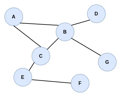
In the graphic above, we can clearly see the components of the formal definition \(G = (V, E)\):

Vertices (\(V\)): The labeled circles (A, B, C, D, E, F, G) represent the set of vertices. Each vertex is a data point or an entity within our system.
Edges (\(E\)): The gray lines connecting the circles represent the set of edges. They define the relationships between vertices. For example, the line between A and B is an edge \(e = (A, B)\), indicating that these two nodes are adjacent.

2. Representations of Graphs

There are two primary ways to translate a visual graph into computer memory: Adjacency Lists and Adjacency Matrices.

A. Adjacency List

The most idiomatic way to represent a graph in Python is a dictionary. Each key is a vertex, and its value is a list of all vertices it is connected to.

graph_dict = { 'A': ['B', 'C'], 'B': ['C', 'D', 'G'], 'C': ['B', 'E'], 'D': ['B'], 'E': ['C', 'F'], 'F': ['E'], 'G': ['B'] }

B. Adjacency Matrix

An adjacency matrix is a 2D array where both rows and columns represent vertices. A value of 1 indicates an edge exists, and 0 indicates no connection.

For our example graph (A-G), the matrix looks like this:

	A	B	C	D	E	F	G
A	0	1	1	0	0	0	0
B	1	0	1	1	0	0	1
C	1	1	0	0	1	0	0
D	0	1	0	0	0	0	0
E	0	0	1	0	0	1	0
F	0	0	0	0	1	0	0
G	0	1	0	0	0	0	0

Tasks:

( Note: In many problems, including those below, we use “node” instead of “vertex”; the terms are interchangeable in graph theory.)

Write a function matrix_to_list(matrix, nodes) that takes a 2D adjacency matrix and a list of node names, and returns an adjacency list (dictionary). Test your function on the graph shown above.
Create an adjacency list as a Python dictionary for a graph with 5 nodes (0, 1, 2, 3, 4) and the following edges: (0, 1), (1, 2), (2, 0), (2, 3), (4, 1), (4, 3).

3. Operations and Complexity

The choice of representation (Adjacency List vs. Adjacency Matrix) significantly impacts the complexity of common operations:

Operation	Adjacency List	Adjacency Matrix
Store Graph	\(O(V + E)\)	\(O(V^2)\)
Add Vertex	\(O(1)\)	\(O(V^2)\)
Add Edge	\(O(1)\)	\(O(1)\)
Query (Are U, V adjacent?)	\(O(V)\)	\(O(1)\)

Note: V = Number of Vertices, E = Number of Edges.

4. Classification of Graphs

Graphs can be classified based on several criteria. Below are the visual comparisons for each type:

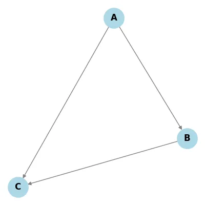
Directionality

Directed	Undirected

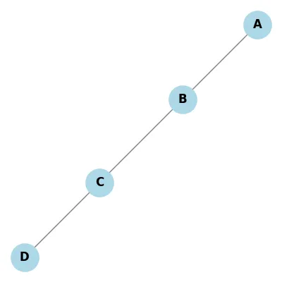
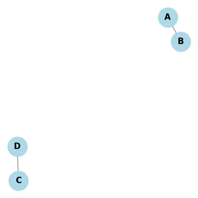
Connectivity

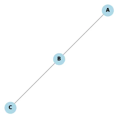
Connected	Disconnected

Cycles

Cyclic	Acyclic

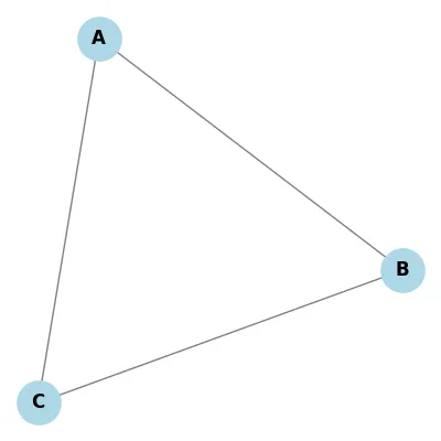Weights

Weighted	Unweighted

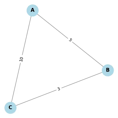5. Basic Graph Implementation (Python Class)

While a dictionary is a great "quick" way to represent a graph, using a class provides better structure for complex operations.

class Graph: def __init__(self): self.adj_list = {} def add_vertex(self, vertex): if vertex not in self.adj_list: self.adj_list[vertex] = [] def add_edge(self, v1, v2, directed=False): self.add_vertex(v1) self.add_vertex(v2) self.adj_list[v1].append(v2) if not directed: self.adj_list[v2].append(v1) def __str__(self): return " ".join([f"{v}: {neighbors}" for v, neighbors in self.adj_list.items()]) # Usage my_graph = Graph() my_graph.add_edge('User1', 'User2') my_graph.add_edge('User2', 'User3') print("Basic Implementation Output:") print(my_graph)

Tasks:

Add a method remove_edge(self, v1, v2) to the Graph class that safely removes a connection between two vertices.
Add a method get_degree(self, vertex) that returns the number of neighbors a vertex has.
Add a method is_valid_path(self, path) that takes a list of nodes (e.g., ['A', 'B', 'C']) and returns True if every consecutive pair in the list is connected by an edge.

6. Graph Traversal Algorithms

We will use the following graph in the visualizations and algorithm tests below:

graph_dict = { 'A': ['B', 'C'], 'B': ['C', 'D', 'G'], 'C': ['B', 'E'], 'D': ['B'], 'E': ['C', 'F'], 'F': ['E'], 'G': ['B'] }

Breadth-First Search (BFS):

Explores all neighbor nodes at the present depth prior to moving on to the nodes at the next depth level. It uses a queue (FIFO) and is ideal for finding the shortest path in unweighted graphs.

Depth-First Search (DFS):

Explores as far as possible along each branch before backtracking. It uses a stack (LIFO) or recursion.

BFS Traversal Implementation

from collections import deque def bfs(graph, start): visited = set() queue = deque([start]) visited.add(start) order = [] while queue: vertex = queue.popleft() order.append(vertex) for neighbor in graph.get(vertex, []): if neighbor not in visited: visited.add(neighbor) queue.append(neighbor) return order print("BFS Order:", bfs(graph_dict, 'A'))

Understanding the BFS Implementation

Breadth-First Search (BFS) explores a graph level by level, starting from a given source node. Here is a step-by-step breakdown of how the code above works:

Initialize Containers:
- We use a set to keep track of all nodes that have already been encountered. This prevents the algorithm from getting stuck in infinite loops (cycles). Using a set data structure allows for very fast verification of whether a node has been visited, with O(1) time complexity.
- BFS uses a Queue (First-In, First-Out) data structure. We start by placing our initial node into this queue.
- This list will store the sequence in which we visit the nodes.
The Main Loop:
- The loop continues as long as there are nodes in the queue.
- We take the oldest node from the front of the queue to explore it.
- Now we add this node to the list that represents the final breadth-first traversal order.
Explore Neighbors:
- We look at all the neighbors of the current node.
- For each neighbor, we check whether it has already been visited.
- If it is a new node, we mark it as visited by adding it to the set and then push it to the back of the queue.

Why use a Queue? By always adding new nodes to the back and taking nodes to explore from the front, we ensure that we visit all nodes at distance 1 before moving to nodes at distance 2, and so on. This property makes BFS ideal for finding the shortest path in unweighted graphs.

DFS Traversal Implementation

Below are two implementations of the DFS algorithm: iterative and recursive. The recursive version is described in detail under the code cells below.

def dfs_iterative(graph, start): visited = set() stack = [start] order = [] while stack: vertex = stack.pop() if vertex not in visited: visited.add(vertex) order.append(vertex) # Add neighbors in reverse order to mimic recursive DFS for neighbor in reversed(graph.get(vertex, [])): if neighbor not in visited: stack.append(neighbor) return order print("DFS Order:", dfs_iterative(graph_dict, 'A'))

def dfs(graph, start, visited=None): if visited is None: visited = [] visited.append(start) for neighbor in graph.get(start, []): if neighbor not in visited: dfs(graph, neighbor, visited) return visited print("DFS Order:", dfs(graph_dict, 'A'))

Understanding the DFS Implementation

Depth-First Search (DFS) explores a graph by going as deep as possible along each branch before backtracking. This implementation uses Recursion, which implicitly utilizes a stack (the call stack).

Function Signature: dfs(graph, start, visited=None):
- We pass the graph and the start node.
- visited is initialized to None and then set to an empty list [] on the first call. This list serves two purposes: tracking visited nodes to avoid cycles and recording the order of traversal.
Visit the Node:
- visited.append(start): As soon as we enter the function for a node, we mark it as visited by adding it to our list.
Recursive Exploration:
- for neighbor in graph.get(start, []): We iterate through all neighbors of the current node.
- if neighbor not in visited: If a neighbor hasn’t been visited yet, we immediately call dfs on that neighbor.
- The "Depth" part: Because we call dfs on the first neighbor before looking at the second neighbor, the algorithm plunges deep into the graph.
Backtracking:
- When a node has no more unvisited neighbors, the function finishes and "returns" to the previous caller (the parent node), which then continues checking its remaining neighbors. This is known as backtracking.

Use Cases: DFS is excellent for tasks like finding connected components, solving puzzles (like mazes), and performing topological sorts in Directed Acyclic Graphs (DAGs).

Tasks:

Modify the bfs function to return a dictionary where keys are nodes and values are their distance (number of edges) from the start node.
Write a function find_path_dfs(graph, start, end) that returns a list of nodes representing a path from start to end, or None if no path exists.
Implement a function has_cycle(graph) that uses either BFS or DFS to detect if there is at least one cycle in the graph.

7. Dijkstra's Shortest Path Algorithm

Dijkstra's Algorithm:
Finds the shortest paths between nodes in a graph. It is a greedy algorithm that works for weighted graphs with non-negative edge weights.

Dijkstra's Algorithm: Step-by-Step Visualization

To understand how Dijkstra's algorithm finds the shortest path, let's trace its execution on a sample graph. We want to find the shortest path from node A to node D.

Step 0: Initial State

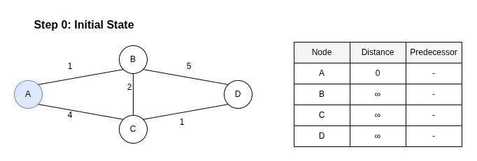
Description:
We start by initializing the distance to the source node (A) as 0 and all other nodes as infinity (∞). At this stage, no predecessors are known. Node A is our starting point.

Step 1: Visit Neighbors of A

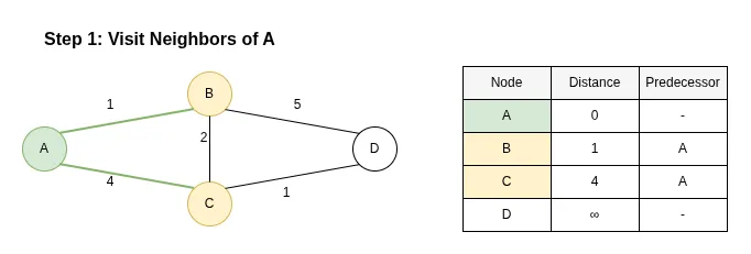
Description:
We extract node A (the node with the smallest distance, 0). We examine its neighbors: B and C.
- The distance to B becomes 0 + 1 = 1 (Predecessor: A).
- The distance to C becomes 0 + 4 = 4 (Predecessor: A).
Node A is now marked as visited (fixed).

Step 2: Visit Neighbors of B

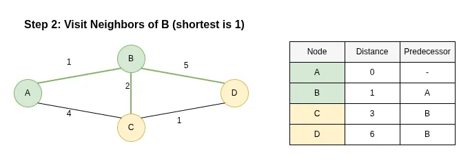
Description:
The next node with the smallest distance is B (dist=1). We explore its neighbors: C and D.
- Updating C: The path A -> B -> C has a length of 1 + 2 = 3. Since 3 is less than the current distance to C (4), we update C's distance to 3 and change its predecessor to B.
- Updating D: The path A -> B -> D has a length of 1 + 5 = 6. We update D's distance to 6 (Predecessor: B).
Node B is now marked as visited.

Step 3: Visit Neighbors of C

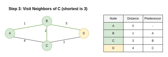
Description:
The next node is C (dist=3). Its neighbor is D.
- Updating D: The path A -> B -> C -> D has a length of 3 + 1 = 4. Since 4 is less than the current distance to D (6), we update D's distance to 4 and change its predecessor to C.
Node C is now marked as visited.

Step 4: Final State

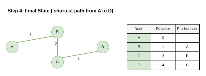
Description:
Finally, we extract node D (dist=4). All nodes have been visited. By following the predecessors backward from D, we find the shortest path: A -> B -> C -> D with a total weight of 4.

import heapq # We define a weighted graph where each edge is a tuple (neighbor, weight) weighted_graph = { 'A': [('B', 1), ('C', 4)], 'B': [('A', 1), ('C', 2), ('D', 5)], 'C': [('A', 4),('B', 2), ('D', 1)], 'D': [('B', 5), ('C', 1)], } def dijkstra(graph, start): # distances will store the current shortest distance to each node distances = {vertex: float('infinity') for vertex in graph} distances[start] = 0 # priority_queue stores (distance, vertex) tuples priority_queue = [(0, start)] while priority_queue: current_distance, current_vertex = heapq.heappop(priority_queue) # If we already found a shorter path to this vertex, ignore this entry if current_distance > distances[current_vertex]: continue for neighbor, weight in graph.get(current_vertex, []): distance = current_distance + weight # If the new distance is shorter than what we've previously recorded, update it if distance < distances[neighbor]: distances[neighbor] = distance heapq.heappush(priority_queue, (distance, neighbor)) return distances print("Dijkstra Shortest Distances from 'A':", dijkstra(weighted_graph, 'A'))

Understanding Dijkstra's Algorithm Implementation

Dijkstra's algorithm finds the shortest path from a starting node to all other nodes in a weighted graph. Unlike BFS, which treats all edges as equal, Dijkstra's algorithm considers the specific weight (or "cost") of each edge.

Setup Distances:
- distances = {vertex: float('infinity') for vertex in graph}: Initially, we don't know any paths, so we set the distance to all nodes to infinity.
- distances[start] = 0: The distance from the start node to itself is zero.
The Priority Queue:
- priority_queue = [(0, start)]: We use a Min-Priority Queue (via heapq). It stores (distance, vertex) tuples.
- The priority queue always yields the node with the smallest known distance to explore next. This greedy strategy ensures we always find the shortest path efficiently.
The Exploration Loop:
- current_distance, current_vertex = heapq.heappop(priority_queue): We extract the "closest" node to the source.
- Optimization Check: if current_distance > distances[current_vertex]: continue. If we have already found a better path to this node, we discard this entry.
Relaxation Step:
- We iterate through each neighbor and its corresponding weight: for neighbor, weight in graph.get(current_vertex, []).
- We calculate the distance via the current node: distance = current_distance + weight.
- if distance < distances[neighbor]: If this new path is shorter than the best one we knew before, we update the distance and push the new path into the priority queue.

Key Insight: Dijkstra's algorithm is essentially a BFS that uses a Priority Queue instead of a regular Queue to handle varying edge weights. It is guaranteed to find the shortest path as long as all edge weights are non-negative.

Other shortest path algorithms

Dijkstra’s algorithm is the most efficient in compute the shortest paths from a single source node to all others, but it requires all edge weights to be non-negative. In contrast, the Bellman–Ford algorithm is more flexible: although slower, it can handle graphs with negative edge weights and can even detect the presence of negative cycles by repeatedly relaxing all edges. Floyd–Warshall takes a different approach altogether, focusing on computing shortest paths between every pair of nodes rather than from a single source. It uses a dynamic programming technique that systematically considers whether passing through intermediate vertices can yield shorter paths. While this makes it very general and easy to implement, it is also the most computationally expensive, with cubic time complexity. In practice, Dijkstra’s algorithm is preferred for performance when its assumptions hold, Bellman–Ford is chosen when negative weights must be supported, and Floyd–Warshall is useful when a complete all-pairs distance matrix is required.

8. When do Developers use Graphs in Practice?

Graphs are ubiquitous in software engineering:

Dependency Management: Package managers (pip, npm) use Directed Acyclic Graphs (DAGs).
Routing Algorithms: Google Maps uses weighted graphs for navigation.
Social Networks: Recommendation engines use graph distance.
Garbage Collection: Identify reachable objects.
Task Scheduling: Airflow and Jenkins model workflows as DAGs.

9. Professional Python Packages for Graph Management

NetworkX: The industry standard for studying complex networks. It is easy to use and provides hundreds of built-in algorithms.
PyG (PyTorch Geometric): Used for Deep Learning on graphs (Graph Neural Networks).
python-igraph: A C-based library with Python bindings, optimized for performance and massive graphs.
Graph-tool: Another high-performance C++ library for Python, known for its speed and advanced visualization.

For production systems, NetworkX is the most popular choice for general-purpose graph analysis:

import networkx as nx # 1. Create a weighted graph G = nx.Graph() G.add_edge('London', 'Paris', weight=450) G.add_edge('Paris', 'Berlin', weight=1050) G.add_edge('London', 'Berlin', weight=1100) # 2. Run a professional algorithm (Shortest Path) shortest_path = nx.shortest_path(G, source='London', target='Berlin', weight='weight') path_length = nx.shortest_path_length(G, source='London', target='Berlin', weight='weight') print(f"Professional Example (NetworkX):") print(f"Shortest path from London to Berlin: {shortest_path}") print(f"Total distance: {path_length} km")

10. Python alternatives to Graphs

Sometimes a graph is overkill or inefficient. Consider these alternatives:

Dictionaries/Hash Maps: For simple 1:1 or 1:N lookups where you don't need traversal.
Sets: For testing membership and uniqueness without relationships.
NumPy Matrices: For dense, static connectivity where you want to use linear algebra (eigenvectors, etc.).

11. Graphs in Machine Learning

Machine Learning is increasingly moving toward non-Euclidean data via Graph Neural Networks (GNNs):

Node Classification: Predicting a property of a node (e.g., is this user a bot?).
Link Prediction: Predicting if an edge should exist (e.g., "You might know this person").
Knowledge Graphs: Modeling structured information (like Google's Knowledge Vault or Wikidata).
Molecular Analysis: Representing molecules as graphs for drug discovery (atoms as nodes, bonds as edges).

In ML, we often convert graphs into numerical data using Adjacency Matrices or Embeddings:

# Machine Learning Context: Adjacency Matrix for a Graph Neural Network (GNN) import numpy as np # Representing a simple friendship graph as a NumPy Matrix for ML models # Nodes: [User0, User1, User2] adj_matrix = np.array([ [0, 1, 0], # User0 is friends with User1 [1, 0, 1], # User1 is friends with User0 and User2 [0, 1, 0] # User2 is friends with User1 ]) # In ML, we might use this matrix to 'propagate' features between friends user_features = np.array([[25], [30], [22]]) # Age of users # Simple aggregation (Graph Convolution): Average friend's age aggregated_features = np.dot(adj_matrix, user_features) print("Machine Learning Concept (Aggregation):") print(f"Sum of friends' ages for each user: {aggregated_features}")

DATA ANALYSIS

Data structures: Graphs

1. What is a Graph?

Visualizing the Concept

2. Representations of Graphs

A. Adjacency List

B. Adjacency Matrix

3. Operations and Complexity

4. Classification of Graphs

Directionality

Connectivity

Cycles

Weights

5. Basic Graph Implementation (Python Class)

6. Graph Traversal Algorithms

Breadth-First Search (BFS):

Depth-First Search (DFS):

BFS Traversal Implementation

Understanding the BFS Implementation

DFS Traversal Implementation

Understanding the DFS Implementation

7. Dijkstra's Shortest Path Algorithm

Dijkstra's Algorithm: Step-by-Step Visualization

Step 0: Initial State

Step 1: Visit Neighbors of A

Step 2: Visit Neighbors of B

Step 3: Visit Neighbors of C

Step 4: Final State

Understanding Dijkstra's Algorithm Implementation

Other shortest path algorithms

8. When do Developers use Graphs in Practice?

9. Professional Python Packages for Graph Management

10. Python alternatives to Graphs

11. Graphs in Machine Learning

Contact details: